
In my last couple of posts on learning to code for coaches (full series with code here), we went through how we can implement Python to obtain data from various sources. In parts 1 and 2 we looked at how you can pull data workout and HRV data straight from your Garmin's fit files. In part 3 we looked at how you can pull data from the web, using Strava's API as an example. In part 4 we looked at how we can pull data from csv exports, using the Pandas library to inspect and clean data from your Training Peaks account. While very important, I have to admit that this process of finding and handling data isn't as sexy as actually using that data to build Machine Learning models! That's what we're going to do in this post. But, before we dive in, some quick definitions. What do I mean when I talk about a "model"? & what do I mean by "Machine Learning".
These 2 concepts of modeling and machine learning are intertwined...
A model is a simplified, abstract representation of the relationship between real world entities.
The key word here is relationship, i.e. a model helps us understand how one thing relates to another. It is through this understanding, that it also enables us to predict "What will happen if..." e.g. if we change one entity but leave the others the same, how will it effect another entity.
Weather is a good example. If I know the time of year, the temperature, the barometer, & the humidity, I have the makings of a model that can predict the likelihood of rain. If it is a good model, I'll be able to manipulate one of those factors to see how it changes the prediction of rain, e.g. if the humidity drops by 10%, how does it affect the chance of rain? Through this modeling we get a deep understanding of the forces involved in a given phenomena.
So, how do we build these models?
Well, one way would be to come in with a mathematical construct of each part. In our world, a good example of this would be modeling how many watts it will take to climb a 4% grade at 25km/h. This is a basic physics equation. If we know the gradient, the weight of the rider and the bike, the wind, the aerodynamic drag, the rolling resistance, we can calculate a physics based model to answer our question. But there is another way of doing it...
We could also get a bunch of different cyclists of different weights and bikes and positions and have them ride up this hill at 25km/h and take note of their average power. Then we could plug the power it took plus all of the other variables that we know - rider weight, bike weight, wind, bike position etc into a computer and we could ask the computer to calculate these relationships for us. Presumably, it would come up with a very similar model to our physics model and thus, in a simplistic sense, we could say that the machine has 'learned' the physics involved in predicting power from these other variables.
This is the essence of machine learning. Rather than feeding the rules to the computer, we feed it data and ask it to figure out the rules.
Of course, the big advantage to this is that we don't need to have to know all of the rules! Even in the simple example above, knowing all of the factors at play to build a physics equation that accurately predicts power output takes significant domain knowledge. And, at the risk of offending my physicist friends, physics is relatively simple when compared to physiology. In physics, the environment that we're dealing with is assumed to be relatively stable. A more realistic example in physiological terms would be to run the same experiment but with each athlete riding their bike uphill on a different planet, where there are is a different gravity being applied to each athlete! In this case, developing the domain knowledge where you can be confident in your predictions is challenging, to say the least, with the traditional approach.
The difficulty in figuring out "the rules" when it comes to exercise physiology should be self-evident in the range of "rules" of training physiology that different coaches have! One rule that is of particular practical interest to the coach is "how aggressively should we ramp the training load?" There are all kinds of simple heuristics that coaches fall back on when it comes to this question - the old "Increase mileage no more than 10% per week" or, the modern version - "'Only' ramp CTL at 10 TSS/wk". Unfortunately, much of coaching is still pervaded by these blanket rules that coaches bring to their programs. Rules that, while they might work for fifty or sixty percent of the athletes that come to the program, leave a large percentage either undertrained or, more commonly, overtrained or injured.
As coaches, rather than come in with some pre-determined "way" that we try to fit our athletes to, a more globally effective strategy is to try to figure out the "way" that works for each athlete & Machine Learning is a great tool for this! If we have a measure of overtraining & we have training load & wellness data for a given athlete, we can feed these variables into a computer & have the computer figure out "the rules" for that individual athlete.
Predicting overtraining in athletes
One of the best indicators that our ramp is too aggressive for a given athlete is when we see a marked drop in heart rate variability. Numerous studies have shown that overtrained athletes exhibit a marked decrease in parasympathetic activity - indicated by significantly lower than normal heart rate variability numbers (e.g. https://onlinelibrary.wiley.com/doi/abs/10.1046/j.1475-0961.2003.00523.x, https://journals.lww.com/cjsportsmed/Abstract/2006/09000/Heart_Rate_Variability,_Blood_Pressure.7.aspx, https://link.springer.com/article/10.1007/s40279-013-0071-8 )
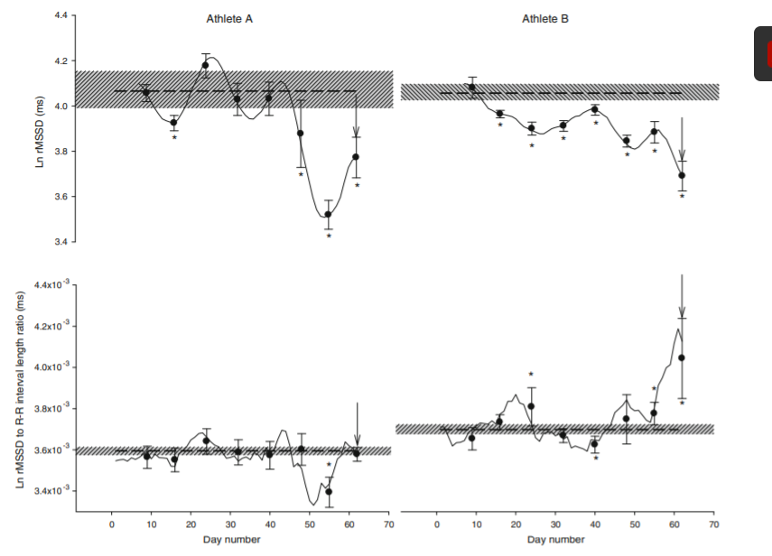
For example, the above diagram from the study in the third link shows the decline in HRV corresponding with declining performance during a bout of overtraining in an elite rower (B)
While it is helpful to have this visibility into the athlete's physiological state to identify when we've exceeded productive load, wouldn't it be great to be able to look ahead into the future to predict what the HRV will be, given the athlete's current state and a given training load, so that we can prevent HRV from dropping BEFORE it actually does?
This "Minority Report" task will be our job here :-), we'll apply some simple Machine Learning to figure out the correct loading "rule" when it comes to the optimal training prescription for one athlete, based on long term historical data for that individual athlete, to adjust our training prescription to minimize the risk of seeing low HRV numbers.
At it's core, this is a math problem....
If we know the athlete's current physiological state - HRV, Sleep metrics, Subjective wellness indicators etc, & we know the athlete's individual load:response relationship, how much load should we give them today to ensure that I don't drive this athlete into overtraining?
Or, in pseudo-math terms...
Today's HRV + Sleep Quality + Mood + x Training Load = acceptable HRV tomorrow (and the day after, and the day after that...)
Now, solve for x.
Importantly, while I'm using HRV as an example of something that you might want to predict, you can build a predictive model for anything you'd like to see more of - watts for a given course, energy, mood, sleep quality etc or, similarly, anything that you want to avoid - fatigue, low energy, injury, illness etc.
Whatever model you are building, the steps are essentially the same..
Step 1: Get the data
To begin with, we need a good amount of individual athlete data. Fortunately, we have plenty of it from the last post (https://www.alancouzens.com/blog/data_wrangling_with_pandas.html). We'll use the same dataframe that we built there to build our model in this post. Let's start by firing that up.
import pandas as pd

data = pd.read_csv("new_improved_metrics.csv")

print(data)
In the above code, we imported that pandas library that we played with in the last blog and then used its read_csv function to read the csv that we generated from our Training Peaks data in the last blog.
This time around, we're going to be using today's metrics to predict how "beat up" we're going to be tomorrow. So, the first thing we need to do is add a separate column to our dataframe for tomorrow's HRV. Let's do that by using the pandas shift function that we introduced in the last post...
data['tomorrows_hrv'] = data['HRV'].shift(-1)
print(data)
Perfect. Now we have a new column that gives tomorrow's hrv number in each row. This will be the variable that we train our data on and teach our model how to predict.
Step 2: Clean the Data
But first, you've probably noticed those weird 'NaN' values above. These 'Not a Number' values represent missing data in our dataframe. Most machine learning algorithms will require "clean" data where all rows have valid values. We have a few options in dealing with these. We could fill these values with the mean or median of the column to create a valid value or we can drop any row that has null values entirely. Let's see how much data we'd be losing to decide which way to go...
data.info()
So, using the pandas info function that we learned about in the last blog, we can see that we have 366 total rows and the features are only missing 4 values at most. In other words, this athlete does a better job than most in being consistent with his data collection! :) So, in this case, the easiest route and the route guaranteed not to pollute our data is to simply drop the rows with missing values. Let's do that...
data = data.dropna()
data.info()
To drop the rows with NaN values from our dataframe, we just use the dropna function.
After doing that, if we run info() again, you can see that we now we have 356 nice, clean, complete rows of data that we can build our model around.
Step 3: Set aside a "test set" to test the error in your model
The next step is an important one. When we're done building our model, we're going to want to test how well it can predict HRV values that it hasn't yet seen. The easiest way to do this is to set aside a portion of our data as a 'test set' that we can use later. So, let's do that by introducing the main python machine learning library that we are going to use in this post - scikit-learn.
In addition to having a ton of different modeling algorithms that we can play with, scikit-learn has a handy function that will automatically split your data into a training set (that we use to train the model) and a test set (that we use to test the model)...
from sklearn.model_selection import train_test_split

data_train, data_test = train_test_split(data, test_size=0.2, random_state=42)
print(f"Training Data: {data_train}")
print(f"Test Data: {data_test}")
In the above code, we applied scikit-learn's train_test_split function to split our dataset in two, setting 20% of our data aside for later testing. We also applied a 'seed' for the random state so that we can replicate that exact same split if needed in the future. This seed can be any number you like but, as a matter of tradition, 42 is selected because 42 is the answer to "the ultimate question of life, the universe and everything" in Hitchhiker's Guide to the Galaxy and, let's face it, most coders are sci-fi geeks :-)
Step 4: Select your model's features
In the last post, we saw how important it is to look at the data prior to modeling. One of the things that it really helps with is determining what features we want to include in our model. Simply looking at how well correlated all of the features are to our target can be really helpful...
corr_matrix = data.corr()
corr_matrix['tomorrows_hrv'].sort_values(ascending=False)
For this athlete, the features most correlated with tomorrow's HRV appear to be how well they slept, the acute training load that they are currently under (negatively correlated - higher load = lower next day HRV) and their self reported life stress. While the acute load (recent average load) seems to be a better predictor than the previous days TSS, since we want our model to be something that we can easily use day-to-day to determine load, let's start with that.
So, let's start by separating our dataset into those features that we think might be good predictors (X) and the variable that we're looking to predict, in this case - tomorrow's HRV (y)
An important note: Don't be too put off by the relatively low R^2 values. When dealing with machine learning, we are often using much larger data sets than is typical in inferential statistics. This leads to lower R^2 values when we look at things on a feature by feature basis. What we look to do in machine learning is to make up for these low R^2 values by a) combining features into one model & b) by not restricting our model to the linear demand of parametric statistics or even, in the case of many ML algorithms, to any known form.
X_train = data_train[['Sleep Quality', 'TSS', 'Stress']]
y_train = data_train['tomorrows_hrv']
X_test = data_test[['Sleep Quality', 'TSS', 'Stress']]
y_test = data_test['tomorrows_hrv']

print(X_train)
print(y_train)
Oops. Houston we have a problem. 'Sleep Quality' is not being found in our list. Weird. If we look a little closer you can see that there is a typo in the key for 'Sleep Quality'. It is misspelled as 'Sleep Qualilty' in our dataframe. Let's fix that by renaming the column...
print(data_train.columns)
data_train.rename(columns={'Sleep Qualilty':'Sleep Quality'}, inplace=True)
data_test.rename(columns={'Sleep Qualilty':'Sleep Quality'}, inplace=True)
print(data_train.columns)
As you can see, it's super easy in pandas to rename a column in your dataset by using pandas inbuilt 'rename' function. OK, now that we've done that, let's try splitting our data into our feature variables and the variable we're trying to predict again...
X_train = data_train[['Sleep Quality','TSS', 'Stress']]
y_train = data_train['tomorrows_hrv']
X_test = data_test[['Sleep Quality','TSS', 'Stress']]
y_test = data_test['tomorrows_hrv']
print(X_train)
print(y_train)
Excellent! We now have our dataframe split into training data (80%) & testing data (20%). And we have each of these sets further split into the predictive features that we want to test (X) and the variable we want to predict(y). We can obviously come back to this step at a later point and try other features to see if they improve our model.
Step 5: Select the right model for the job
Now we're ready for the fun part - building a model. Once you've done all of the preceding steps to get some nice clean data to work with, you'll be surprised by just how easy scikit-learn makes this part of the process!
Scikit-learn offers a number of different machine learning algorithms to choose from depending on the type of machine learning we are doing...
Classification algorithms - predict what class or category a given input fits into.
Regression algorithms - predict a continuous variable, i.e a number
Clustering algorithms - take a bunch of inputs and group them together according to similarity of features
So which one are we using here?
We're predicting HRV - a continuous numeric variable, so we're dealing with a regression problem. Now, even within the subset of regression algorithms, scikt-learn has a number to choose from. It's always good policy to try the simplest model first to at least get a good baseline. For regression, one of the simplest models is linear regression. This is super easy to implement with scikit-learn...
from sklearn.linear_model import LinearRegression

linear_model = LinearRegression()
linear_model.fit(X_train, y_train)
Step 6: Take your model for a test-drive
That's it! We now have a working model that will predict what an athlete's HRV will be the next day if we give it Sleep Quality, atl, Stress & Mood.
Let's take it for a spin...
prediction = linear_model.predict([[5, 100, 1]])
print(f"Predicted HRV: {prediction}")
So, if we have the really positive scores of - a sleep quality of 5/5, a training load of 100 TSS and a reported stress level of 1/5, our predicted HRV for the next day is 10.0. Given the really good sleep quality and low stress and pretty mild training load, we'd predict that a HRV scor eof 10.0 is probably pretty good for this athlete. Let's see how it ranks compared to their long term data...
data['HRV'].describe()
By running the describe() function that we introduced in the last blog, we get some nice summary statistics of a given feature. Comparing our athlete's 10.0 HRV with their mean value of 9.78, we can see it is very good! In fact, it's almost in the top 75% of all values! Looking at this, our athlete could probably handle some more load! Let's put 300TSS into our model and see what it does to the system..
prediction = linear_model.predict([[5, 300, 1]])
print(f"Predicted HRV: {prediction}")
A slight hit but, with those positive morning metrics - great sleep quality and a very low stress day, I predict he'll handle it well. Now, what if those morning metrics aren't so good?
prediction = linear_model.predict([[1, 300, 4]])
print(f"Predicted HRV: {prediction}")
Now, with poor sleep quality of 1/5 and a high stress level of 4/5, our heavy training load of 300TSS is predicted to push this athlete's HRV below the bottom 25% of all values. That's not great. Maybe, under these conditions of super high stress, we should give him a rest day of zero TSS...
prediction = linear_model.predict([[1, 0, 4]])
print(f"Predicted HRV: {prediction}")
Ah, much better! Still on the low side of normal but getting closer to the athlete's normal HRV. Let's roll with that rest day today.
Step 7: Assess your model's error & ways to improve it
Now, before we place too much trust in our model, it pays to sit it down at the proverbial school desk and test it. You'll remember that we set aside part of our data, that our model hasn't seen yet, as a test set for this very purpose. So, let's see how it does in predicting data that it hasn't seen....
import numpy as np
from sklearn.metrics import mean_squared_error
predictions = linear_model.predict(X_test)
linear_model_mse = mean_squared_error(y_test, predictions)
linear_model_rmse = np.sqrt(linear_model_mse)
print(f"Error: {linear_model_rmse}")
To get the error of our model, scikit-learn comes to the rescue again with their mean_squared_error function. The root mean square error is a common metric used to assess the error of regression models. It provides an intuitive way to look at the error as it tells us an absolute error range (on the same scale as the metrics that we're predicting) that a majority of samples will fall between.
A root mean square error of 0.40, while not horrible, is clearly not great either. This means that if our model predicts 9.6, the 'true' value will likely fall between 9.2 and 10.0. If we look at the athlete's data, that's a pretty big range. From below the worst 25% of values to about the top 60%. Or, from a really bad HRV number to a decent one. But fear not, we're just getting started, there are a number of ways that we can improve the predictive power of our model:
We can add more features from our dataset. To keep things simple, we only started with 3 features - sleep quality, TSS and stress. In the "real world" these models can have hundreds of features. If you add more features above (CTL, ATL, mood etc), you will see the error come down. If you're playing around with the Colab notebook, you can change the code above and play around with adding more features to see the impact that it has on the model error.
We can add better features to our dataset. You'll remember from the correlation analysis that longer term training load metrics (ATL, CTL) better correlated with HRV than pure daily load. Additionally, different types of training are going to have a more pronounced effect on HRV than any measure of pure load. We could amend our data set to include time in zone and different sports to give more fidelity than a single load number can offer. I talk more about some of the limits of using TSS based models here (https://alancouzens.com/blog/Banister_v_Neural_Network.html)
We could apply a more complex, non-linear, algorithm like a decision tree, a random forest or even a neural network to our problem. The non-linear bit will significantly improve our model. As I explain in the link above, physiological processes tend to be non-linear, i.e. the HRV doesn't tend to decrease linearly with load but, instead, hits a breakpoint at a certain point. This non-linearity can't be reflected in the linear model that we're using above.
I'll look at some of these more complex algorithms in my next post.
Until then...
Train smart,
AC